Real-time data processing experts
Use Calabash GUI, click on the “Pipeline” heading on top of the window. The Pipeline page becomes the current page. Set the data system to “lake_finance” and click on the big green “Create Pipeline” button.
Enter “payment-p3” as the name of the pipeline. Select the Kafka system named “lf-kafka” and enter the pipeline user name “pl.”
Since the values in the source topic “converted-log1” are not text, you must define the source schema. See below.
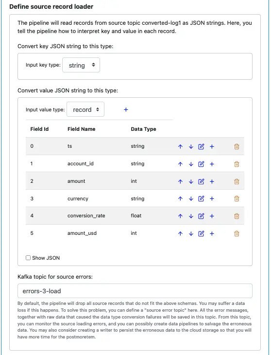
It is a good practice to set an error topic for the source. The error topic “errors-3-load” will help you capture any errors. The errors will most likely be due to an incorrect schema you have defined here. The messages in the error topic will help you diagnose problems.
For our tutorial, if you have not added more records to the topics “log1,” “clean-log1,” and “converted-log1,” there should be no errors in the source loader.
Next, we define processors. Click on the small blue plus sign next to “Define pipeline processors.” Enter information for the first processor as follows.
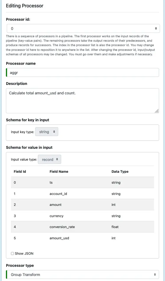
You cannot modify the input schemas because they are the key and value schemas of the source loader. We have defined them earlier.
Select “Group Transform” as the processor type.
The group transform first performs a group-by-key, then calculates aggregate values for each group. The output key is the same as that of the input. But the output value will have new fields. See below.
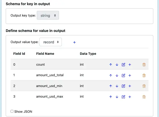
We will calculate the following aggregate values for each group:
The group transform processor must buffer data before performing aggregation. We must define a time window size for the buffering.

In the tutorial, we set the buffering time to 180 seconds. In practice, you must make a judgment based on the dynamic behavior of your data stream.
Next, we start to define the processing functions. There will be no preprocessing function in this processor.
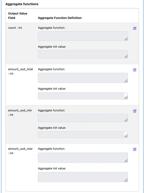
For each output value field, we must define two functions. One is an aggregate function, and the other is an initial-value function. Right now, neither is defined for all the fields. See below.
Click on the edit button for the field “count: int,” and enter the code as the following screenshot.
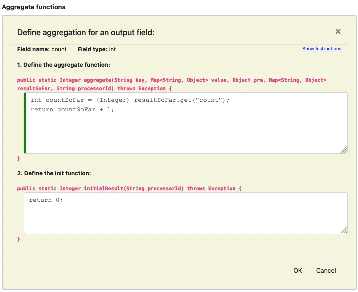
The implementation tells the pipeline how to calculate the count for the group. It returns the initial value of 0. Then every time the aggregate function is called, it adds 1 to the intermediate “count” result.
The init function is called only once. But the aggregate one is called once for each record in the group. The intermediate, partial result is stored in the variable “resultSoFar.” Please click on the “Show Instruction” link to expand the instructions to learn more details.
Click OK to return back to the processor editor.
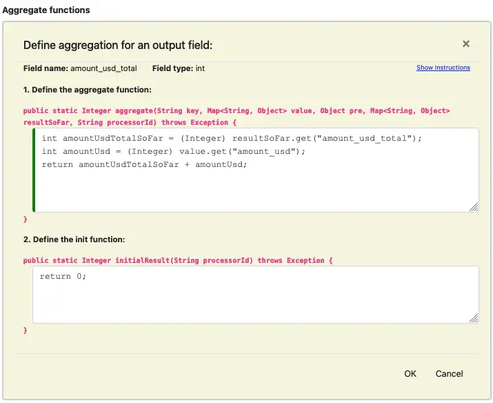
Let’s see another aggregate function editor. This is for the output field “amount_usd_total.”
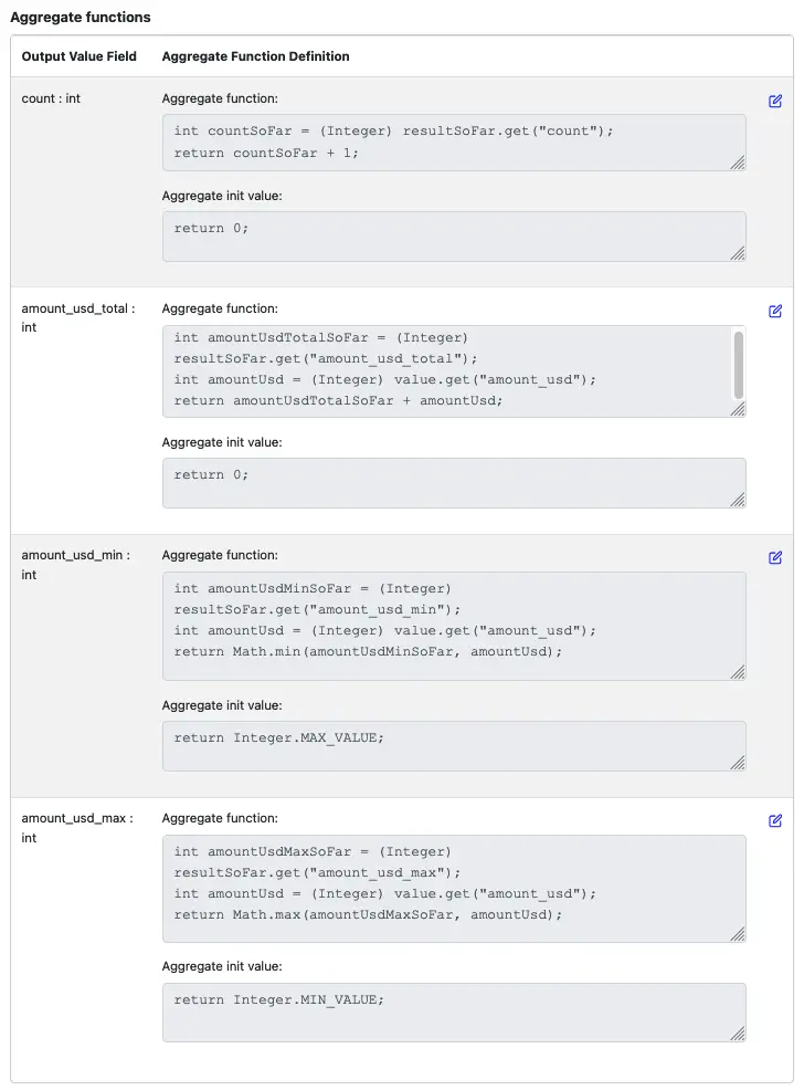
Similarly, you can enter code for the remaining two output value fields. The output functions in the processor editor should look like this.
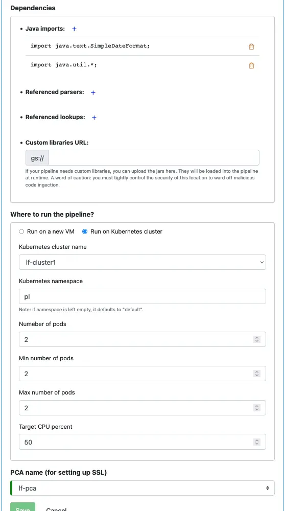
There is no change in the “Dependencies” section, so take the default.
Set the location for running this pipeline to the cluster we have deployed in the earlier tutorial track.
Last but not least, set the PCA to “lf-pca.” Then click on the “Save” button to persist the pipeline to the Calabash repository.
